Calculus
The word Calculus comes from Latin meaning "small stone",
Because it is like understanding something by looking at small pieces.
Differential Calculus cuts something into small pieces to find how it changes.
Integral Calculus joins (integrates) the small pieces together to find how much there is.
|  |
Introduction to Calculus
Calculus is all about changes.
 |
Sam and Alex are travelling in the car ... but the speedometer is broken.
|
Alex:
|
"Hey Sam! How fast are we going now?"
| |
Sam:
|
"Wait a minute ..."
"Well in the last minute we went 1.2 km, so we are going:"
1.2 km/minute x 60 minutes in an hour = 72 km/h
| |
Alex:
| "No, Sam! Not our average for the last minute, or even the last second, I want to know our speed RIGHT NOW." | |
Sam:
|
"OK, let us measure it up here ... at this road marker... NOW!"
"OK, we were AT the road marker for zero seconds, and the distance was ... zero meters!"
The speed is 0m / 0s = 0/0 = I Don't Know!
"I can't calculate it Sam! I need to know some distance over some time, and you are saying the time should be zero? Can't be done."
|
That is pretty amazing ... you'd think it is easy to work out the speed of a car at any point in time, but it isn't.
Even the speedometer of a car (when it works!) just shows us an average of how fast we were going for the last short amount of time.
How About Getting Real Close
But our story is not finished yet!
Sam and Alex get out of the car, because they have arrived on location. Sam is about to do a stunt:
 |
Sam will do a jump off a 20 m building.
Alex, as photographer, asks:
"How fast will you be falling after 1 second?"
Sam uses this simplified formula to find the distance fallen:
d = 5t2
- d = distance fallen, in meters
- t = time from jump, in seconds
But how fast is that? Speed is distance over time:
| Speed = | distance |
| time |
So at 1 second:
| Speed = | 5 m | = 5 m/s |
| 1 second |
"BUT", says Alex, "again that is an average speed, since you started the jump, ... I want to know the speed at exactly 1 second, so I can set up the camera properly."
 |
Well ... at exactly 1 second the speed is:
|
So again Sam has a problem.
Think about it ... how do we figure out a speed at an exact instant in time?
What is the distance? What is the time difference?
They are both zero, giving us nothing to calculate with!
But Sam has an idea ... invent a time so short it won't matter.
Sam won't even give it a value, and will just call it "Δt" (called "delta t").
So Sam works out the difference in distance between t and t+Δt
At 1 second Sam has fallen
d = 5t2 = 5 × (1)2 = 5 m
At (1+Δt) seconds Sam has fallen
d = 5t2 = 5 × (1+Δt)2 m
We can expand (1+Δt)2:
| (1+Δt)2 | = (1+Δt)(1+Δt) |
| = 1 + 2Δt + (Δt)2 |
And we get:
| d | = 5 × (1+2Δt+(Δt)2) m |
| = 5 + 10Δt + 5(Δt)2 m |
So between 1 second and (1+Δt) seconds the distance fallen is:
| Change in d | = (5 + 10Δt + 5(Δt)2) − 5 m |
| = 10Δt + 5(Δt)2 m |
Now divide that distance by time to get the speed:
| Speed | = 10Δt +5(Δt)2 mΔt s |
| = 10 + 5Δt m/s |
So the speed is 10 + 5Δt m/s, and Sam thinks about that Δt value ... he wants Δt to be so small it won't matter ... so he imagines it shrinking towards zero and he gets:
Speed = 10 m/s
Wow! Sam got an answer!
Sam: "I will be falling at exactly 10 m/s"
Alex: "I thought you said you couldn't calculate it?"
Sam: "That was before I used Calculus!"
Yes, indeed, that was Calculus.
The word Calculus comes from Latin meaning "small stone".
Because it is like understanding something by looking at small pieces.
Because it is like understanding something by looking at small pieces.
Differential Calculus cuts something into small pieces to find how it changes.
Integral Calculus joins (integrates) the small pieces together to find how much there is.
And Differential Calculus and Integral Calculus are like inverses of each other, just like multiplication and division are inverses.
Sam used Differential calculus to cut time and distance into such small pieces that a pure answer came out.
So ... was Sam's result just luck? Does it work for other things?
Let's try doing this for the function y = x3
This is going to be very similar to the previous example, but it will be just a slope on a graph, no one has to jump for this one!
Example: What is the slope of the function y = x3 at x=1 ?

Try It Yourself!
Go to the Slope of a Function page, put in the formula "x^3", then try to find the slope at the point (1,1).
Zoom in closer and closer and see what value the slope is heading towards.
Conclusion
Calculus is about changes.
Differential calculus cuts something into small pieces to find how it changes.
Integral calculus joins (integrates) the small pieces together to find how much there is.
Limits (An Introduction)
Approaching ...
Sometimes we can't work something out directly ... but we can see what it should be as we get closer and closer!
Example:
Now 0/0 is a difficulty! We don't really know the value of 0/0 (it is "indeterminate"), so we need another way of answering this.
So instead of trying to work it out for x=1 let's try approaching it closer and closer:
Example Continued:
We are now faced with an interesting situation:
- When x=1 we don't know the answer (it is indeterminate)
- But we can see that it is going to be 2
We want to give the answer "2" but can't, so instead mathematicians say exactly what is going on by using the special word "limit"
The limit of (x2−1)(x−1) as x approaches 1 is 2
And it is written in symbols as:
 So it is a special way of saying, "ignoring what happens when we get there, but as we get closer and closer the answer gets closer and closer to 2"
As a graph it looks like this:
So, in truth, we cannot say what the value at x=1 is.
But we can say that as we approach 1, the limit is 2.
|  |
Test Both Sides!
It is like running up a hill and then finding the pathis magically "not there"...
... but if we only check one side, who knows what happens?
So we need to test it from both directions to be sure where it "should be"!
Example Continued
When it is different from different sides
 How about a function f(x) with a "break" in it like this:
The limit does not exist at "a"
We can't say what the value at "a" is, because there are two competing answers:
How about a function f(x) with a "break" in it like this:
The limit does not exist at "a"
We can't say what the value at "a" is, because there are two competing answers:
- 3.8 from the left, and
- 1.3 from the right
But we can use the special "−" or "+" signs (as shown) to define one sided limits:
- the left-hand limit (−) is 3.8
- the right-hand limit (+) is 1.3
And the ordinary limit "does not exist"
Are limits only for difficult functions?
Limits can be used even when we know the value when we get there! Nobody said they are only for difficult functions.
Example:
Approaching Infinity
 | Infinity is a very special idea. We know we can't reach it, but we can still try to work out the value of functions that have infinity in them. |
Let's start with an interesting example.
Question: What is the value of 1∞ ?
Answer: We don't know!
| Question: What is the value of 1∞ ? |
| Answer: We don't know! |
Why don't We know?
The simplest reason is that Infinity is not a number, it is an idea.
So 1∞ is a bit like saying 1beauty or 1tall.
Maybe we could say that 1∞= 0, ... but that is a problem too, because if we divide 1 into infinite pieces and they end up 0 each, what happened to the 1?
In fact 1∞ is known to be undefined.
But We Can Approach It!
So instead of trying to work it out for infinity (because we can't get a sensible answer), let's try larger and larger values of x:
|  |
Now we can see that as x gets larger, 1x tends towards 0
We are now faced with an interesting situation:
- We can't say what happens when x gets to infinity
- But we can see that 1x is going towards 0
We want to give the answer "0" but can't, so instead mathematicians say exactly what is going on by using the special word "limit"
The limit of 1x as x approaches Infinity is 0
And write it like this:
In other words:
As x approaches infinity, then 1x approaches 0
When you see "limit", think "approaching"
It is a mathematical way of saying "we are not talking about when x=∞, but we know as x gets bigger, the answer gets closer and closer to 0".
Solving!
We have been a little lazy so far, and just said that a limit equals some value because it looked like it was going to.
Continuous Functions
A function is continuous when its graph is a single unbroken curve ...
 ... that you could draw without lifting your pen from the paper.
That is not a formal definition, but it helps you understand the idea.
Here is a continuous function:
... that you could draw without lifting your pen from the paper.
That is not a formal definition, but it helps you understand the idea.
Here is a continuous function:
... that you could draw without lifting your pen from the paper.Examples
So what is not continuous (also called discontinuous) ?
Look out for holes, jumps or vertical asymptotes (where the function heads up/down towards infinity).
 |  |  | ||
| Not Continuous | Not Continuous | Not Continuous | ||
| (hole) | (jump) | (vertical asymptote) |
Domain
A function has a Domain.
In its simplest form the domain is all the values that go into a function.
|  |
A function might be continuous or not, depending on its Domain!
Example: 1/(x-1)
So when a function is continuous within its Domain, it is a continuous function.
More Formally !
We can define continuous using Limits (it helps to read that page first):
A function f is continuous when, for every value c in its Domain:
f(c) is defined, and:
"the limit of f(x) as x approaches c equals f(c)"
The limit says:
"as x gets closer and closer to c
then f(x) gets closer and closer to f(c)"
And we have to check from both directions:
"the limit of f(x) as x approaches c equals f(c)"
then f(x) gets closer and closer to f(c)"
| as x approaches c (from left) then f(x) approaches f(c) |  | |
| AND as x approaches c (from right) then f(x) approaches f(c) |  |
If we get different values from left and right (a "jump"), then the limit does not exist!
How to Use:
Make sure that, for all x values:
- f(x) is defined
- and the limit at x equals f(x)
Here are some examples:
Example: f(x) = (x2-1)/(x-1) for all Real Numbers
Let us change the domain:
Example: g(x) = (x2-1)/(x-1) over the interval x<1
Example: How about this piecewise function:
But:

Example: How about the piecewise function absolute value:
Derivatives (Differential Calculus)
The Derivative is the "rate of change" or slope of a function.
Introduction to Derivatives
It is all about slope!
| Slope = |
|  |
We can find an average slope between two points.
|  | |
But how do we find the slope at a point?
There is nothing to measure!
|  | |
But with derivatives we use a small difference ...
... then have it shrink towards zero.
|  |
Let us Find a Derivative!
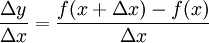
We will use the slope formula:
| Slope = | Change in Y | = | Δy |
| Change in X | Δx |
to find the derivative of a function y = f(x)
x changes from x to x+Δx
y changes from f(x) to f(x+Δx)
y changes from f(x) to f(x+Δx)
Follow these steps:
| • Fill in this slope formula: |
| ||||||||
| • Simplify it as best we can, | |||||||||
| • Then make Δx shrink towards zero. | |||||||||
Here we go:
Example: the function f(x) = x2
We write dx instead of "Δx heads towards 0", so "the derivative of" is commonly written  x2 = 2x
"The derivative of x2 equals 2x"
or simply "d dx of x2 equals 2x"
"The derivative of x2 equals 2x"
or simply "d dx of x2 equals 2x"
What does x2 = 2x mean?
It means that, for the function x2, the slope or "rate of change" at any point is 2x.
So when x=2 the slope is 2x = 4, as shown here:
Or when x=5 the slope is 2x = 10, and so on.
Let's try another example.
Example: What is x3 ?
Have a play with it using the Derivative Plotter.
Derivatives of Other Functions
We can use the same method to work out derivatives of other functions (like sine, cosine, logarithms, etc).
But in practice the usual way to find derivatives is to use:
Derivative Rules
But in practice the usual way to find derivatives is to use:
Derivative Rules
Example: what is the derivative of sin(x) ?
Using the rules can be tricky!
Example: what is the derivative of cos(x)sin(x) ?
So that is your next step: learn how to use the rules.
Notation
"Shrink towards zero" is actually written as a limit like this:

"The derivative of f equals the limit as Δx goes to zero of f(x+Δx) - f(x) over Δx"
Or sometimes the derivative is written like this (explained on Derivatives as dy/dx):


The process of finding a derivative is called "differentiation".
You do differentiation ... to get a derivative.
"The derivative of f equals the limit as Δx goes to zero of f(x+Δx) - f(x) over Δx"
You do differentiation ... to get a derivative.
Derivative Rules
The Derivative tells us the slope of a function at any point.
The derivatives of many functions are well known. Here are some useful rules to help you work out the derivatives of more complicated functions (with examples below). Note: the little mark ’means "Derivative of".
Common Functions Function Derivative Constant c 0 x 1 Square x2 2x Square Root √x (½)x-½ Exponential ex ex ax ax(ln a) Logarithms ln(x) 1/x loga(x) 1 / (x ln(a)) Trigonometry (x is in radians) sin(x) cos(x) cos(x) −sin(x) tan(x) sec2(x) sin-1(x) 1/√(1−x2) cos-1(x) −1/√(1−x2) tan-1(x) 1/(1+x2) Rules Function Derivative Multiplication by constant cf cf’ Power Rule xn nxn−1 Sum Rule f + g f’ + g’ Difference Rule f - g f’ − g’ Product Rule fg f g’ + f’ g Quotient Rule f/g (f’ g − g’ f )/g2 Reciprocal Rule 1/f −f’/f2 Chain Rule
(as "Composition of Functions") f º g (f’ º g) × g’ Chain Rule (in a different form) f(g(x)) f’(g(x))g’(x)
"The derivative of" is also written
| Common Functions | Function | Derivative |
|---|---|---|
| Constant | c | 0 |
| x | 1 | |
| Square | x2 | 2x |
| Square Root | √x | (½)x-½ |
| Exponential | ex | ex |
| ax | ax(ln a) | |
| Logarithms | ln(x) | 1/x |
| loga(x) | 1 / (x ln(a)) | |
| Trigonometry (x is in radians) | sin(x) | cos(x) |
| cos(x) | −sin(x) | |
| tan(x) | sec2(x) | |
| sin-1(x) | 1/√(1−x2) | |
| cos-1(x) | −1/√(1−x2) | |
| tan-1(x) | 1/(1+x2) | |
| Rules | Function | Derivative |
| Multiplication by constant | cf | cf’ |
| Power Rule | xn | nxn−1 |
| Sum Rule | f + g | f’ + g’ |
| Difference Rule | f - g | f’ − g’ |
| Product Rule | fg | f g’ + f’ g |
| Quotient Rule | f/g | (f’ g − g’ f )/g2 |
| Reciprocal Rule | 1/f | −f’/f2 |
| Chain Rule (as "Composition of Functions") | f º g | (f’ º g) × g’ |
| Chain Rule (in a different form) | f(g(x)) | f’(g(x))g’(x) |
"The derivative of" is also written
Examples
Example: what is the derivative of sin(x) ?
Power Rule
Example: What is x3 ?
Example: What is (1/x) ?
Multiplication by constant
Example: What is 5x3 ?
Sum Rule
Example: What is the derivative of x2+x3 ?
Difference Rule
It doesn't have to be x, we can differentiate with respect to, for example, v:
Example: What is  (v3−v4) ?
Sum, Difference, Constant Multiplication And Power Rules
Example: What is  (5z2 + z3 − 7z4) ?
Product Rule
Example: What is the derivative of cos(x)sin(x) ?
Reciprocal Rule
Example: What is (1/x) ?
Chain Rule
Example: What is sin(x2) ?
Example: What is (1/sin(x)) ?
Example: What is (5x−2)3 ?
Derivatives as dy/dx
Derivatives are all about change ...
... they show how fast something is changing (called the rate of change) at any point.
In Introduction to Derivatives (please read it first!) we looked at how to do a derivative usingdifferences and limits.
Here we look at doing the same thing but using the "dy/dx" notation (also called Leibniz's notation) instead of limits.
We start by calling the function "y":
y = f(x)
1. Add Δx
When x increases by Δx, then y increases by Δy
y + Δy = f(x + Δx)
When x increases by Δx, then y increases by Δy
y + Δy = f(x + Δx)
2. Subtract the Two Formulas
From:
y + Δy = f(x + Δx)
Subtract:
y = f(x)
To Get:
y + Δy - y = f(x + Δx) - f(x)
Simplify:
Δy = f(x + Δx) - f(x)
| From: |
y + Δy = f(x + Δx)
| |
| Subtract: |
y = f(x)
| |
| To Get: |
y + Δy - y = f(x + Δx) - f(x)
| |
| Simplify: |
Δy = f(x + Δx) - f(x)
|
3. Rate of Change
To work out how fast (called the rate of change) we divide by Δx:
To work out how fast (called the rate of change) we divide by Δx:
4. Reduce Δx close to 0
We can't let Δx become 0 (because that would be dividing by 0), but we can make it head towards zero and call it "dx":
Δx  dx
You can also think of "dx" as being infinitesimal, or infinitely small.
Likewise Δy becomes very small and we call it "dy", to give us:
dx
You can also think of "dx" as being infinitesimal, or infinitely small.
Likewise Δy becomes very small and we call it "dy", to give us:
We can't let Δx become 0 (because that would be dividing by 0), but we can make it head towards zero and call it "dx":
Δx dx
You can also think of "dx" as being infinitesimal, or infinitely small.
Likewise Δy becomes very small and we call it "dy", to give us:
Try It On A Function
Let's try f(x) = x2
Let's try f(x) = x2
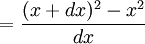
f(x) = x2 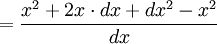
Expand (x+dx)2 
Simplify (x2-x2=0) 
Simplify fraction 
dx goes towards 0
| f(x) = x2 | |||
| Expand (x+dx)2 | |||
| Simplify (x2-x2=0) | |||
| Simplify fraction | |||
| dx goes towards 0 |
Second Derivative
(Read about derivatives first if you don't already know what they are!)
A derivative basically gives you the slope of a function at any point.
The "Second Derivative" is the derivative of the derivative of a function. So:
- Find the derivative of a function
- Then take the derivative of that
A derivative is often shown with a little tick mark: f'(x)
The second derivative is shown with two tick marks like this: f''(x)
The second derivative is shown with two tick marks like this: f''(x)
| A derivative can also be shown as: | dy | , and the second derivative shown as: | d2y |
| dx | dx2 |
Distance, Speed and Acceleration
A common real world example of this is distance, speed and acceleration:
| So: | Example Measurement | |||||
| Distance: | s | 100 m | ||||
| First Derivative is Speed: |
| 10 m/s | ||||
| Second Derivative is Acceleration: |
| 2 m/s2 |
And the third derivative (how acceleration changes over time) is called "Jolt" ... !
Differentiable
Differentiable means that the derivative exists ...
... and it must exist for every value in the function's domain.
Domain
In its simplest form the domain is
all the values that go into a function | |
But what about this:
Testing
We can test any value "c" by finding if the limit exists:
| lim h→0 | f(c+h) − f(c) |
| h |
A good way to picture this in your mind is to think:
As I zoom in, does the function tend to become a straight line?
The absolute value function stays pointy even when zoomed in.
Other Reasons
Here are a few more examples:
 |
The Floor and Ceiling Functions are not differentiable at integer values, as there is a discontinuity at each jump. But they are differentiable elsewhere.
|
 |
The Cube root function x(1/3)
Its derivative is (1/3)x-(2/3) (by the Power Rule)
At x=0 the derivative is undefined, so x(1/3) is not differentiable.
|
 |
At x=0 the function is not defined so it makes no sense to ask if they are differentiable there.
To be differentiable at a certain point, the function must first of all be defined there!
|
 |
As we head towards x = 0 the function moves up and down faster and faster, so we cannot find a value it is "heading towards".
So it is not differentiable.
|
Different Domain
But we can change the domain!

Why Bother?
Because when a function is differentiable we can use all the power of calculus when working with it.
Continuous
When a function is differentiable it is also continuous.
Differentiable ⇒ Continuous
But a function can be continuous but not differentiable. For example the absolute value function is actually continuous (though not differentiable) at x=0.
Taylor Series
A Taylor Series is an expansion of a function into an infinite sum of terms, like these ones:
| Taylor Series expansion | As Sigma Notation |
 | |
 | |
 | |
 |
(There are many more)
Approximations
You can use the first few terms of a Taylor Series to get an approximate value for a function.
Here we show better and better approximations for cos(x). The red line is cos(x), the blue is the approximation (try plotting it yourself) :
| 1 − x2/2! |  |
| 1 − x2/2! + x4/4! |  |
| 1 − x2/2! + x4/4! − x6/6! |  |
| 1 − x2/2! + x4/4! − x6/6! + x8/8! |  |
(You can also see the Taylor Series in action at Euler's Formula for Complex Numbers.)
What is this Magic?
How can you turn a function into a series of power terms like this?
Well, it isn't really magic. First you say you want to have this:
f(x) = c0 + c1(x-a) + c2(x-a)2 + c3(x-a)3 + ...
Then choose a value "a", and work out the values c0 , c1 , c2 , ... etc
It is done using derivatives ...
Quick review: a derivative gives you the slope of a function at any point.
You must know the derivatives of your function f(x) and these basic derivative rules :
- The derivative of a constant is 0
- The derivative of x is 1
- The derivative of xn is nxn-1 (Example: the derivative of x3 is 3x2)
We will use the little mark ’ to mean "derivative of".
OK, let's start:
To get c0, choose x=a so all the (x-a) terms become zero, leaving you with:
f(a) = c0
So c0 = f(a)
To get c1, take the derivative of f(x):
f’(x) = c1 + 2c2(x-a) + 3c3(x-a)2 + ...
With x=a all the (x-a) terms become zero:
f’(a) = c1
So c1 = f’(a)
To get c2, do the derivative again:
f’’(x) = 2c2 + 3×2×c3(x-a) + ...
With x=a all the (x-a) terms become zero:
f’’(a) = 2c2
So c2 = f’’(a)/2
In fact, a pattern is emerging. Each term is
- the next higher derivative ...
- ... divided by all the exponents so far multiplied together (for which we can use factorial notation, for example 3! = 3×2×1)
And we get:
Now we have a way of finding our own Taylor Series: keep taking derivatives and divide by n! each time.
Try that for sin(x) yourself, it will help you to learn.
Or try it on another function of your choosing. The key thing is that you be able to take derivatives of your function f(x).
Note: A Maclaurin Series is a Taylor Series where a=0, so all the examples we have been using so far can also be called Maclaurin Series.
Integration (Integral Calculus)
Integration can be used to find areas, volumes, central points and many useful things.
Introduction to Integration
Integration is a way of adding slices to find the whole.
Integration can be used to find areas, volumes, central points and many useful things. But it is easiest to start with finding the area under the curve of a function like this:
What is the area under y = f(x) ?
Slices
We could calculate the function at a few points and add up slices of width Δx like this (but the answer won't be very accurate):
|  | |
We can make Δx a lot smaller and add up many small slices(answer is getting better):
|  | |
And as the slices approach zero in width, the answer approaches thetrue answer.
We now write dx to mean the Δx slices are approaching zero in width.
|  |
That is a lot of adding up!
But we don't have to add them up, as there is a "shortcut". Because ...
... finding an Integral is the reverse of finding a Derivative.
(So you should really know about Derivatives before reading more!)
Like here:
You will see more examples later.
Notation
The symbol for "Integral" is a stylish "S"
(for "Sum", the idea of summing slices): |  |
After the Integral Symbol we put the function we want to find the integral of (called the Integrand),
and then finish with dx to mean the slices go in the x direction (and approach zero in width).
And here is how we write the answer:
Plus C
We wrote the answer as x2 but why + C ?
It is the "Constant of Integration". It is there because of all the functions whose derivative is 2x:

The derivative of x2+4 is 2x, and the derivative of x2+99 is also 2x, and so on! Because the derivative of a constant is zero.
So when we reverse the operation (to find the integral) we only know 2x, but there could have been a constant of any value.
So we wrap up the idea by just writing + C at the end.
Tap and Tank

Integration is like filling a tank from a tap.
The input (before integration) is the flow rate from the tap.
Integrating the flow (adding up all the little bits of water) gives us thevolume of water in the tank.
Imagine the flow starts at 0 and gradually increases (maybe a motor is slowly opening the tap).

As the flow rate increases, the tank fills up faster and faster.
With a flow rate of 2x, the tank fills up at x2.
We have integrated the flow to get the volume.
We can do the reverse, too:

Imagine you don't know the flow rate.
You only know the volume is increasing by x2.
You only know the volume is increasing by x2.
We can go in reverse (using the derivative, which gives us the slope) and find that the flow rate is 2x.
 |
So Integral and Derivative are opposites.
|
We can write that down this way:
The integral of the flow rate 2x tells us the volume of water:
| ∫2x dx = x2 + C | |
And the slope of the volume increase x2+C gives us back the flow rate:
|

And hey, we even get a nice explanation of that "C" value ... maybe the tank already has water in it!
- The flow still increases the volume by the same amount
- And the increase in volume can give us back the flow rate.
Which teaches us to always add "+ C".
Other functions
Well, we have played with y=2x enough now, so how do we integrate other functions?
If we are lucky enough to find the function on the result side of a derivative, then (knowing that derivatives and integrals are opposites) we have an answer. But remember to add C.

But a lot of this "reversing" has already been done (see Rules of Integration).
Knowing how to use those rules is the key to being good at Integration.
So get to know those rules and get lots of practice.
Learn the Rules of Integration and Practice! Practice! Practice!
(there are some questions below)
(there are some questions below)
Definite vs Indefinite Integrals
We have been doing Indefinite Integrals so far.
A Definite Integral has actual values to calculate between (they are put at the bottom and top of the "S"):
 |  | |
| Indefinite Integral | Definite Integral |
Integration Rules
Integration
Integration can be used to find areas, volumes, central points and many useful things. But it is often used to find the area underneath the graph of a function like this:
| |
The integral of many functions are well known, and there are useful rules to work out the integral of more complicated functions, many of which are shown here.
There are examples below to help you.
| Common Functions | Function | Integral |
|---|---|---|
| Constant | ∫a dx | ax + C |
| Variable | ∫x dx | x2/2 + C |
| Square | ∫x2 dx | x3/3 + C |
| Reciprocal | ∫(1/x) dx | ln|x| + C |
| Exponential | ∫ex dx | ex + C |
| ∫ax dx | ax/ln(a) + C | |
| ∫ln(x) dx | x ln(x) − x + C | |
| Trigonometry (x in radians) | ∫cos(x) dx | sin(x) + C |
| ∫sin(x) dx | -cos(x) + C | |
| ∫sec2(x) dx | tan(x) + C | |
| Rules | Function | Integral |
| Multiplication by constant | ∫cf(x) dx | c∫f(x) dx |
| Power Rule (n≠-1) | ∫xn dx | xn+1/(n+1) + C |
| Sum Rule | ∫(f + g) dx | ∫f dx + ∫g dx |
| Difference Rule | ∫(f - g) dx | ∫f dx - ∫g dx |
| Integration by Parts | See Integration by Parts | |
| Substitution Rule | See Integration by Substitution | |
Examples
Power Rule
Multiplication by constant
Sum Rule
Difference Rule
Sum, Difference, Constant Multiplication And Power Rules
Integration by Parts
Integration by Parts is a special method of integration that is often useful when two functions are multiplied together, but is also helpful in other ways.
You will see plenty of examples soon, but first let us see the rule:
∫u v dx = u∫v dx −∫u' (∫v dx) dx
- u is the function u(x)
- v is the function v(x)
As a diagram:

And let us get straight into an example:

So we followed these steps:
- Choose u and v
- Differentiate u: u'
- Integrate v: ∫v dx
- Put u, u' and ∫v dx here: u∫v dx −∫u' (∫v dx) dx
- Simplify and solve
In English, to help you remember, ∫u v dx becomes:
(u integral v) minus integral of (derivative u, integral v)
Let's try some more examples:


Well, that was a spectacular disaster! It just got more complicated.
Maybe we could choose a different u and v?

The moral of the story: Choose u and v carefully!
Choose a u that gets simpler when you differentiate it and a v that doesn't get any more complicated when you integrate it.
A helpful rule of thumb is I LATE. Choose u based on which of these comes first:
- I: Inverse trigonometric functions such as sin-1(x), cos-1(x), tan-1(x)
- L: Logarithmic functions such as ln(x), log(x)
- A: Algebraic functions such as x2, x3
- T: Trigonometric functions such as sin(x), cos(x), tan (x)
- E: Exponential functions such as ex, 3x
And here is one last (and tricky) example:
Where Did "Integration by Parts" Come From?
It is based on the Product Rule for Derivatives:
(uv)' = uv' + u'v
Integrate both sides and rearrange:
∫(uv)' dx = ∫uv' dx + ∫u'v dx
uv = ∫uv' dx + ∫u'v dx
∫uv' dx = uv − ∫u'v dx
Some people prefer that last form, but I like to integrate v' so the left side is simple:
∫uv dx = u∫v dx − ∫u'(∫v dx) dx
Integration by Substitution
"Integration by Substitution" (also called "u-substitution") is a method to find an integral, but only when it can be set up in a special way.
The first and most vital step is to be able to write our integral in this form:

Note that we have g(x) and its derivative g'(x)
Like in this example:

Here f=cos, and we have g=x2 and its derivative of 2x
This integral is good to go!
When our integral is set up like that, we can do this substitution:

Then we can integrate f(u), and finish by putting g(x) back as u.
Like this:

So ∫cos(x2) 2x dx = sin(x2) + C worked out really nicely! (Well, I knew it would.)
This method only works on some integrals of course, and it may need rearranging:
Now we are ready for a slightly harder example:

And how about this one:

So there you have it.
In Summary
When we can put an integral in this form:
Then we can make u=g(x) and integrate ∫f(u) du
And finish up by re-inserting g(x) where u is.
Differential Equations
In our world things change, and describing how they change often ends up as a Differential Equation: an equation with a function and one or more of its derivatives:
Differential Equations
A Differential Equation is an equation with a function and one or more of its derivatives:
Example: an equation with the function y and its derivative dydx
Solving
We solve it when we discover the function y (or set of functions y).
There are many "tricks" to solving Differential Equations (if they can be solved!), but first: why?
Why Are Differential Equations Useful?
In our world things change, and describing how they change often ends up as a Differential Equation:

Differential Equations can describe how populations change, how heat moves, how springs vibrate, how radioactive material decays and much more. They are a very natural way to describe many things in the universe.
What To Do With Them?
We try to solve them by turning the Differential Equation into a simpler Algebra-style equation (without the differential bits) so we can do calculations, make graphs, predict the future, and so on.

So Differential Equations are great at describing things, but need to be solved to be useful.
More Examples of Differential Equations
The Verhulst Equation
Simple harmonic motion
In Physics, Simple Harmonic Motion is a type of periodic motion where the restoring force is directly proportional to the displacement. An example of this is given by a mass on a spring.
Classify Before Trying To Solve
OK, we want to solve them, but how?

Over the years wise people have worked out special methods to solve some typesof Differential Equations.
It is like travel: different kinds of transport have solved how to get to certain places.
Is it near, so we can just walk? Is there a road so we can take a car? Is it over water so we need a ship? Or is it in another galaxy and we just can't get there yet?
So our first task is to classify the Differential Equation.
Ordinary or Partial
The first major grouping is:
- "Ordinary Differential Equations" (ODEs) have a single independent variable (like y)
- "Partial Differential Equations" (PDEs) have two or more independent variables.
We are learning about Ordinary Differential Equations here!
Order and Degree
Next we work out the Order and the Degree:
Order
The Order is the highest derivative (is it a first derivative? a second derivative? etc):
Degree
The degree is the exponent of the highest derivative.
Be careful not to confuse order with degree. Some people use the word order when they mean degree!
Linear
It is Linear when the variable (and its derivatives) has no exponent or other function put on it.
So no y2, y3, √y, sin(y), ln(y) etc, just plain y (or whatever the variable is).
More formally a Linear Differential Equation is in the form:
| dy | + P(x)y = Q(x) |
| dx |
Solving
OK, we have classified our Differential Equation, the next step is solving.
Example: an equation with the function y and its derivative dydx
Example: an equation with the function y and its derivative dydx
Example: an equation with the function y and its derivative dydx
Separation of Variables
Separation of Variables is a special method to solve some Differential Equations
A Differential Equation is an equation with a function and one or more of itsderivatives:
Example: an equation with the function y and its derivative dydx
When Can I Use it?
Separation of Variables can be used when:
All the y terms (including dy) can be moved to one side of the equation, and
All the x terms (including dx) to the other side.
Method
Three Steps:
- Step 1 Move all the y terms (including dy) to one side of the equation and all the x terms (including dx) to the other side.
- Step 2 Integrate one side with respect to y and the other side with respect to x. Don't forget "+ C" (the constant of integration).
- Step 3 Simplify
We used y and x, but the same method works for other variable names, like this:
There are other equations that follow this pattern such as continuous compound interest.
More Examples
OK, on to some different examples of separating the variables:
A harder example:
An even harder example: the famous Verhulst Equation
Solution of First Order Linear Differential Equations
You might like to read about Differential Equations and Separation of Variables first!
A Differential Equation is an equation with a function and one or more of its derivatives:
Example: an equation with the function y and its derivative dydx
Here we will look at solving a special class of Differential Equations called First Order Linear Differential Equations
First Order
They are "First Order" when there is only dydx , not d2ydx2 or d3ydx3 etc
Linear
A first order differential equation is linear when it can be made to look like this:
| dy | + P(x)y = Q(x) |
| dx |
Where P(x) and Q(x) are functions of x.
To solve it there is a special method:
- We invent two new functions of x, call them u and v, and say that y=uv.
- We then solve to find u, and then find v, and tidy up and we are done!
And we also use the derivative of y=uv (see Derivative Rules (Product Rule) ):
| dy | = u | dv | + v | du |
| dx | dx | dx |
Steps
Here is a step-by-step method for solving them:
- 1. Substitute y = uv, and
intody = u dv + v du dx dx dx dy + P(x)y = Q(x) dx - 2. Factor the parts involving v
- 3. Put the v term equal to zero (this gives a differential equation in u and x which can be solved in the next step)
- 4. Solve using separation of variables to find u
- 5. Substitute u back into the equation we got at step 2
- 6. Solve that to find v
- 7. Finally, substitute u and v into y = uv to get our solution!
Let's try an example to see:
What is the meaning of those curves? They are the solution to the equation dydx − yx = 1
In other words:
Anywhere on any of those curves
the slope minus yx equals 1
the slope minus yx equals 1
Let's check a few points on the c=0.6 curve:
Estmating off the graph (to 1 decimal place):
| Point | x | y | Slope (dydx) | dydx − yx |
|---|---|---|---|---|
| A | 0.6 | −0.6 | 0 | 0 − −0.60.6 = 0 + 1 = 1 |
| B | 1.6 | 0 | 1 | 1 − 01.6 = 1 − 0 = 1 |
| C | 2.5 | 1 | 1.4 | 1.4 − 12.5 = 1.4 − 0.4 = 1 |
Why not test a few points yourself? You can plot the curve here.
Perhaps another example to help you? Maybe a little harder?
And one more example, this time even harder:
Homogeneous Differential Equations
A Differential Equation is an equation with a function and one or more of itsderivatives:
Example: an equation with the function y and its derivative dydx
Here we look at a special method for solving "Homogeneous Differential Equations"
Homogeneous Differential Equations
A first order Differential Equation is Homogeneous when it can be in this form:
dydx = F( yx )
We can solve it using Separation of Variables but first we create a new variable v = yx
v = yx is also y = vx
And dydx = d (vx)dx = v dxdx + x dvdx (by the Product Rule)
Which can be simplified to dydx = v + x dvdx
Using y = vx and dydx = v + x dvdx we can solve the Differential Equation.
An example will show how it is all done:
Another example:
And one last example:
No comments:
Post a Comment